Building A New NBA Team 'The Vegas Bandits' through Analytics

Authors:

Muhammad Murtadha Ramadhan, Firas Rasyid, Jaden Mullin, Evan Benham, Calvin Huang

Background:

The NBA, as the premier basketball league in the world, has always been a lucrative business for cities. One of those aspiring cities is Las Vegas. Over the years, the allure and glitz of Vegas has brought teams from various leagues: WNBA moved the Aces in 2018, NFL infamously moved the Raiders from Oakland, and Formula 1 had a race in Vegas recently. There are rumblings that the MLB also intends to move the Oakland A’s to Sin City.

The NBA also has plans for Las Vegas. The newly introduced In-Season Tournaments will have their semi-finals and finals in Las Vegas. Moreover, the organization is planning to either move or create a new expansion team in the city. Various investors–notably Shaquille O’Neal and LeBron James–are sounding their interest to turn the vision of having an NBA team in Vegas into reality. The Oak View Group, one of the leading investors, was recently cited to build a $10 Billion NBA arena if the expansion goes through.

Clearly, there is a lot riding on the success of the future NBA Vegas team. A winning Vegas team will create a legacy, build a strong and passionate fan base, and become a launch pad for future growth and success. That is why roster-building is especially important for the new team: having a successful group of players from the get-go will pay dividends in the future.

Although the process could take years in the making, our team assumes that the team starts in the 2023/2024 season. Thus, the new team needs players to fill up their roster; we are using player performance metrics to find the best players in each position and their backups. We dive deep into the data, finding which metrics correlate most to winning basketball. Moreover, we also consider the salary cap.

So, to summarize, our problem statement is: Which players are we going to choose for a Las Vegas NBA team based on their performance metrics in the 2022-2023 season, given limited budget?

Methodology:

The overall steps taken for the analysis are as follows:

1. Prepare the dataset
2. Separate players into two groups based on their team standings
3. Use T-Test to find which metrics matter most to winning
4. Use optimization by weighting the shortlisted metrics and considering salary cap

Datasets:

Overall, we used 4 datasets: NBA Standings, Per Game Metrics, Advanced Metrics, and Salary Data. All of the datasets are from the 2022-2023 Season.

Our assumptions:

1. Use regular season data, as not all teams participate in the Playoffs
2. Assume only NBA players playing in the 2022-2023 Season are available
3. Assume that all players are available to procure
4. The salary cap is a hard limit; no team can exceed it

For NBA Standings, Per Game Metrics, and Advanced Metrics, we took data from https://www.basketball-reference.com/ which uses official NBA data. For salary, we use https://hoopshype.com/ . All of the data are publicly available. Per Game Metrics and Advanced Metrics are used to find which metrics correlate most to the team's winnings, which we got from NBA Standings data. Moreover, we use the Salary Data as our source for players’ salaries. The granularity of the data is per player, and all the data are data that were gathered by the end of the season. Thus, a player who only plays for 1 game but scored a lot can have a few metrics skewed, for example, %FG (field goal scored/total field goal attempts). Moreover, a lot of data was already being processed (through a set of formulas). Finally, the data obviously is going to skew towards healthy players. For example, LaMelo Ball only played 36 out of 82 games due to a fractured ankle injury. This could be mitigated by taking into account previous seasons’ stats, but due to limited time and resources, we only evaluated one season.

Analysis

Winning Stats

The first step to forming a new team is to decide the player stats that most correlate to team wins. When deciding how to best quantify how good a team is at winning, our team thought of two possible routes. The first would be to look at a current NBA team’s overall stats, or the stats of all the players combined, to see how they work together to bring home wins for their teams. The second route would be to look at individual player’s overall stats for the previous season and see how those stacked up against players in the same position. We decided to go for the second approach since our newly drafted team will most likely not incorporate synergies seen in the previous season and the fact that currently there is no robust stat that quantifies player synergies.

Next the dataset needed to be validated and cleaned. The first problem that needed to be addressed were duplicate player rows. If a player transferred to a different team mid season, the stats would be split into different rows for each team they were in. To remedy this problem, players that had multiple rows, had new total rows made summing up all rows they appeared in. The team they ended the season on was listed as their team for the season. A similar problem occurred with player positions, as players who moved teams could also switch positions during the switch. For example during his trade to the Brooklyn Nets, Mikal Bridges went from playing small forward to the shooting guard. The same process was followed as with team switches, with the player’s position being listed as the one he finished the season in. Although these changes may lead to bias down the line, it was decided that this would be the best course of action to minimize the loss of player data in processes that will be described later.

To compare players in each position two comparison groups needed to be made in order to perform a t test later on. Because the aim of any NBA team is to win the most games, the players were divided into those that were a part of the top 15 teams by wins and those in the bottom 15 teams. These groups were further filtered so only the players in the top 25% of minutes played would remain. This would ensure that only players with high contribution to their team winning would be a part of the analysis. For most positions this meant players with less than 1700 minutes played during the course of the season were not considered in our analysis. One consideration that must be taken into account from this method is that by filtering by minutes played, those that were injured during last season will not be looked at, However, if we aim to create a team for the 2023/24 season we agreed it would be ebay to move forward with players that will be ready to field at the beginning of the season and have a good track record from the previous season.

After splitting the dataset into two groups data frames were created for each position, so comparisons would be made between players in one position. For each position roughly 30 players were kept after filtering for minutes played. With the n between comparison groups being less than 30, being 15 in the top and bottom groups, a t test was chosen to test for significant differences in each stat line. Basic stats like 2 point shots made and total assists were tested, as well as advanced stats like OWS or offensive win share. The alpha level of the tests was set at 0.05 and the null hypothesis was generally that players from the bottom teams had the same average as those in the top team for the stat being tested. The alternative was that players from the top teams would have higher averages in the stat of interest. Below is an example of the comparison of the 2 point shots made for centers and the t test performed with the resulting test statistic and p value.

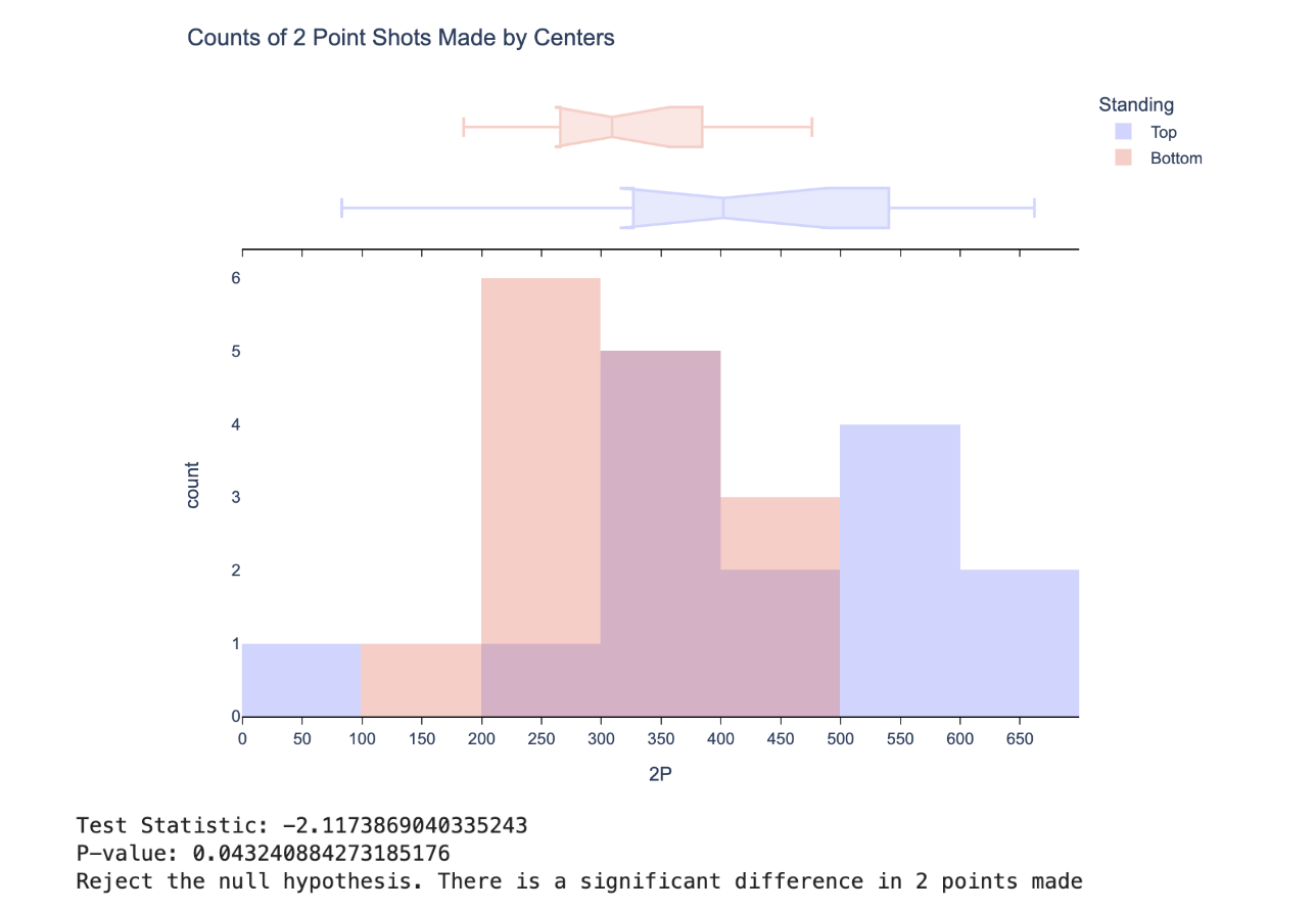
After performing t tests on all player stats for all five positions, all of the win share stats such as OWS, or offensive win share, were found to be significant. This result was expected and these stats were not used in our final list of winning due to winshare stats being heavily tied to the overall performance of the team in addition to the abilities of the individual player. Other than those stats the remaining stats that were listed as significant were used.

For centers, it was found that 2P, DBPM, BPM, and VORP yielded significant differences between groups. 2P is the number of 2 pointers made over the course of the season. DBPM or defensive box plus/minus, is an estimate of a player’s value to their team while on defense per 100 possessions. Finally VORP or value over replacement player, is a box value similar to DBPM of the points per 100 team possessions a player has over a replacement player (set at -2.0) and translated to an average team.

For small forwards, it was found that TOV, ORB, DRB, and TRB all yielded significant differences between groups. TOV is the number of turnovers or times a player lost possession of the ball to the other team. ORB, DRB, and TRB all have to do with the number of rebounds in a season being offensive, defensive, and total rebounds respectively. For shooting guards, it was found that 3P, 3P%, and 3PAr yielded significant differences. All three of these stats have to do with how well a player made 3 point shots being 3 points made, successful 3 point shot percentage, and the percent of all field goals that were 3 pointers respectively.

For power forwards, eFG%, TS%, DBPM, BPM, and VORP were found to have significant differences. eFG% is the effective percentage of field goals made with added weight to 3 point shots due to the increased value. TS% is true shooting percentage is similar to eFG%, but also takes free throws into account. BPM is similar to the aforementioned DBPM but is a measure of point value given to a team per 100 possessions rather than only measuring defensive value.

Finally, for point guard 3P% and STL were found to have significant differences. The STL stat tracks the amount of times a player stole the ball from a player from the opposing team.

Weighting Stats and Ranking Players

#[3P, 3P%, 3PAr, DWS, WS, WS/48]
weights = {'3P': 0.166, '3P%': 0.167, '3PAr': 0.167, 'DWS': 0.167, 'WS': 0.167, 'WS/48': 0.166}

# Normalize the stats and calculate weighted score
for stat in weights.keys():
    max_value = sg2[stat].max()
    sg2.loc[:, stat + '_norm'] = sg2[stat] / max_value

sg2.loc[:, 'Weighted_Score'] = sum([sg2[stat + '_norm'] * weight for stat, weight in weights.items()])

# Rank players
ranked_sg2 = sg2.sort_values('Weighted_Score', ascending=False)

# Display the top ranked players
ranked_sg2[['Player_adv', 'Tm_adv', 'Pos_adv', 'Weighted_Score']]

After identifying the key winning statistics for each position, we determined that it would be appropriate to build a model (Figure 2) to calculate a weighted score for each player to fairly rank them among their positions. To begin developing the model, we first assigned an equal weighting to the key statistics within each of the five positions. Since the statistical category was already identified to be statistically significant, we determined that this weighting methodology would ultimately allow us to value each statistic equally. After determining the weighting methodology, the statistics of each player were normalized to scale all the statistics to a 0 – 1 range, which allowed for a fair comparison between them. The weighted score was calculated by taking the sum of the products of each normalized statistic and the corresponding weight for each player. This resulted in ranking the players from the best to worst, descending from the highest calculated score. Additionally, the formulation for shooting guards noted within figure 2, was also replicated for the other four positions.

Top 5 Ranking Center

Top 5 Ranking Point Forward

Top 5 Ranking Point Guard

Top 5 Ranking Shooting Forward

Top 5 Ranking Shooting Guard

Figures 3 – 7 displays the top five players in their respective position ranked based on their weighted score. In comparison to the NBA, the results are fairly consistent with publicly published power rankings of NBA players.

Player Selection with Linear Optimization

After obtaining the weighted performance score and ranking all the potential players, the quadrant mapping is conducted to get a brief sense of which potential players that might be chosen.

Potential Players Scatter Plot with Quadrant Mapping

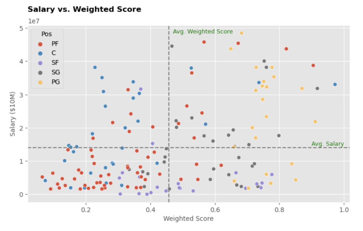
Seeing the scatter plot with quadrant area, we expect to hire players that lie on the bottom right quadrant who are higher in weighted score but lower in salary cost. Seeing the plot deeper, there are quite many player options in the bottom right quadrant except for the Power Forward position.

Then, we run linear optimization to decide which players to hire to our roster with detailed formulations as follows:

Decision variables:

• Which players to hire for each position

Objectives:

• Maximizing the weighted score of players hired

Constraints:

• For each position, the total players that can be hired are 2 players
• Total salaries for all players hired can’t exceed $123.655 million with the reference to NBA official source
• Referring to research by Samford University, total salaries percentage for each position should be at most (of total salaries):
  • PG: 23.10%
  • SG: 20.98%
  • SF: 21.47%
  • PF: 16.50%
  • Center: 17.96%
• Maximum age is 30 years old for each player hired since we build a new team and with the long term vision to develop young players further as well

Then, the formulated is translated into python code with Gurobi library below:

all_final_player = pd.DataFrame()

for pos in list(optimization_player_final['Pos'].unique()):
    import pandas as pd
    from gurobipy import Model, GRB
    I = optimization_player_final[optimization_player_final['Pos'] == pos].index
    mod = Model()
    x = mod.addVars(I, vtype = GRB.BINARY, name = 'x')
    mod.setObjective(sum(x[i]*optimization_player_final.loc[i, 'Weighted_Score'] for i in I), sense = GRB.MAXIMIZE)

    # total players per position
    mod.addConstr(sum(x[i] for i in I) == 2)

    # budget per position
    mod.addConstr(sum(x[i]*optimization_player_final.loc[i, 'Salary'] for i in I) <= salary_budget.loc[pos, 'budget'])
    
    # age
    for i in I:
        if optimization_player_final.loc[i, 'Age'] > 30:
            mod.addConstr(x[i] == 0)
    
    # mod.write('10-nba.lp')
    # %cat 10-nba.lp
    mod.setParam('OutputFlag', False)
    mod.optimize()
    mod.objval

    player = []
    
    for i in I:
        if x[i].x == 1:
            player.append(i)
    
    chosen = optimization_player_final.loc[player]
            
    all_final_player = pd.concat([all_final_player, chosen], sort=False)
            
all_final_player.sort_values(by = ['Pos', 'Weighted_Score'])

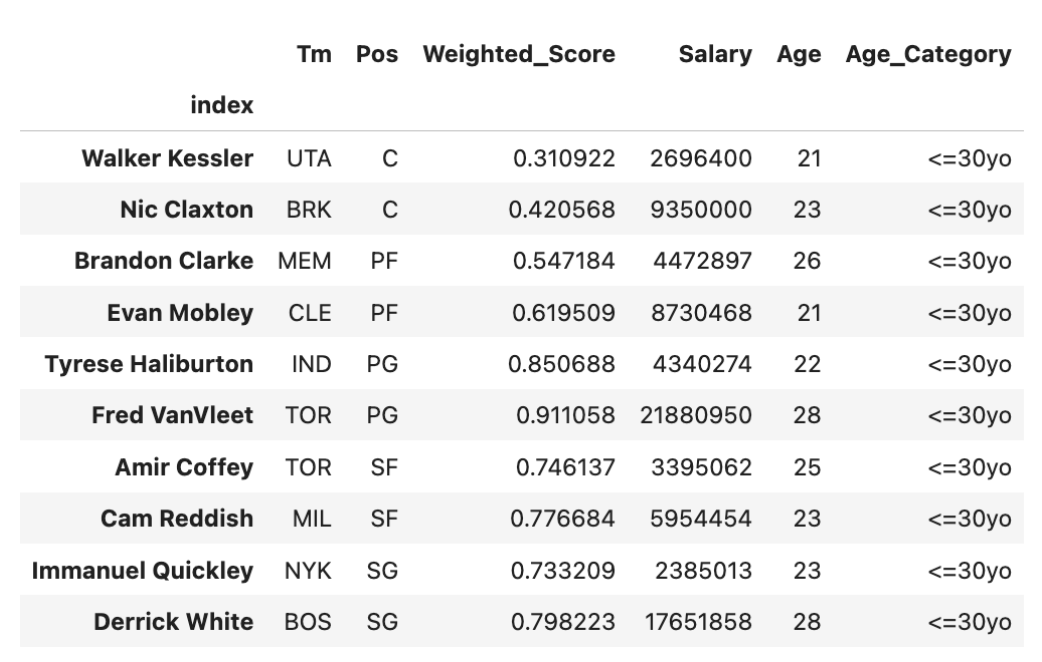
The linear optimization results in 10 selected players with 2 players in each position with details below:

Selected Players List with Their Weighted Performance Score, Salary, and Age

Selected Player Photos

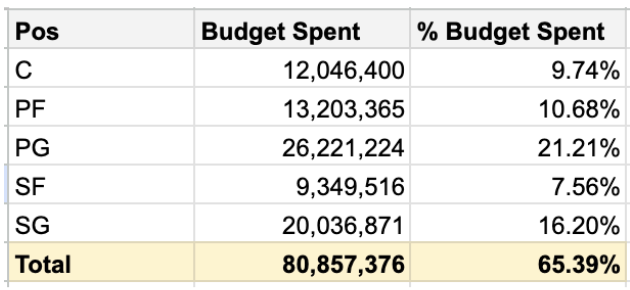
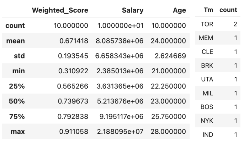
The optimization result leads to obtaining the most optimal total weighted score of 6.7142 and average weighted score of 0.671. In addition, the all selected players to hire would only use 65% of total budget cap to hire all selected players. The details of budget spent breakdown of each position as follows:

Budget Spent Breakdown by Position

In brief descriptive statistics, The age of selected player is in the range of 21 y.o to 28 y.o and with salary range of $2,385,013 to $21,880,950. Ultimately, almost all players to hire are from different teams except 2 players from Toronto Raptors.

Descriptive Statistics of All Selected Players

Conclusion

In all, our model gave us a final team that we believe optimizes the Las Vegas Bandits’ ability to compete with any team in the NBA and allows them to utilize their salary budget in the most efficient way possible.

For each position that we analyzed, we had some expectations, or hypotheses, about which statistics would be statistically significant and which wouldn’t. These expectations were a product of our collective understanding of basketball and were intuitive in nature. For example, looking at the point guard position, we understood that point guard is historically seen as the “quarterback” of the court, distributing the ball to other players to facilitate scoring opportunities. Because of this, we believed that assists and assist percentage would be statistically significant for point guards from top half teams versus bottom half teams. It made intuitive sense to us that better teams would have point guards who can distribute the ball more effectively than worse teams, thus making their assist statistics more significant. However, as can be seen with the results for many of our positions, this wasn’t the case. While at first we found this puzzling, especially for the point guard position, as we discussed our analysis, we came to the realization that, in the case of a point guard, being able to distribute the ball effectively is a prerequisite to the position, and therefore one should expect that any point guard has these skills, regardless of what team they play for.

Moreover, we posited that the stats that we did find statistically significant at each position for better teams versus worse teams show how players on better teams are able to contribute in other areas of the game, in areas that aren’t normally thought of for their given position, and in turn have a positive impact on their team overall. As another example, for small forwards, this is a position that relies a lot on scoring, so our inclination was that two point percentage, three point percentage, points per game, and other scoring stats would likely be significant. However, it turned out that total rebounds, offensive rebounds, and defensive rebounds were all significant, signaling that small forwards on better teams are able to extend their game to other areas aside from scoring, to rebounding, to help their team more than small forwards on worse teams. Due to their ability to both score and rebound, small forwards on better teams contribute more to the game than their counterparts on inferior teams, and this flexibility in their game contributes more to the team overall, therefore impacting their team’s ability to win games. In the case of small forwards specifically, while obviously the ability to score is impactful on a team’s chances of winning, the ability for small forwards on superior teams to rebound gives their teams more scoring opportunities. In this way, small forwards on better teams find more ways to impact the game than their counterparts on worse teams, and therefore, in theory, contribute more to their team’s ability to win. While we are ultimately limited in our ability to truly measure whether one statistic or another contributes the most to a team’s ability to win games, we believe that the model we constructed gives us the best chance to capture this potential. We believe in the validity of our results because our methodology took into account all available NBA players, from all teams, but we also included certain thresholds for players to qualify for our analysis. For example, when determining which players to analyze at any given position, we wanted to make sure that we were analyzing players who contribute to their team consistently, either as a starter or as a bench player. Therefore, we determined that only players who contributed at or more than the 75th percentile of minutes played at their position in the 2022-2023 season would be analyzed. We came to this decision because we believed that players who did not meet this threshold, perhaps only playing several games over the course of the season, could skew our analysis due to their high potential of outlier statistics. By having a minutes played threshold, we ensured that we were only analyzing players who consistently impacted their team over the season, and that the statistics we were analyzing were more standardized and less biased in nature. Moreover, we wanted to have a homogenous method to split our players into those from “good” teams and those from “bad” teams. To achieve this, we took all of the players from teams that finished in the top 50% of teams for the 2022-2023 season as the “good” group, and vice versa for the “bad” group. This method ensured that we were accounting for all teams in the NBA and their players. We also made sure to have roughly equal sample sizes of players from good teams and bad teams for each position group. We wanted to have equal sample sizes to ensure the fairness of our analysis.

Overall, we were able to successfully determine for each position group which statistics were significantly different between players from good teams versus bad teams, and theorized that these statistics distinguish how players from good teams are able to adapt their games and contribute more to their team overall than players from bad teams, thus contributing to their team’s ability to win games. We are limited by the fact that there is currently no guaranteed statistic that measures a player’s ability to contribute to their team’s ability to win, and ultimately it is the combination of many statistics that determine whether a certain player contributes positively or negatively to their team overall. However, we believe that our sound methodology, measuring all available data at our disposal, breaking teams into good versus bad, and determining thresholds for our final analyses, point to the fact that our findings show how players on winning teams contribute more to their team than players on losing teams, giving an inclination into which types of statistics may be more impactful to a team’s winning percentage at any given position.

References:

• https://www.basketball-reference.com/
• https://hoopshype.com/
• https://www.samford.edu/sports-analytics/fans/2019/An-Analysis-of-NBA-Teams-Spending-by-Position-for-the-Upcoming-Season